Aspect

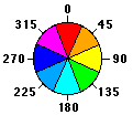
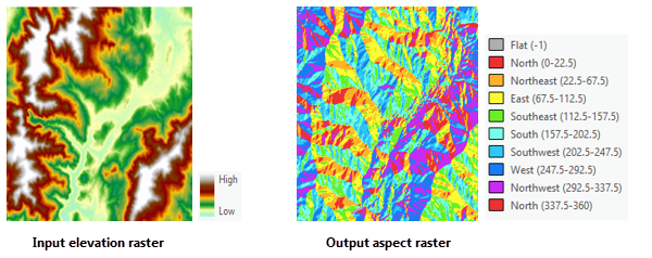
The Aspect surface parameter identifies the direction the downhill slope faces. The value of each cell in the output raster indicates the compass direction the surface faces at that location. It is measured clockwise in degrees from 0 (due north) to 360 (again due north), coming full circle. Flat areas having no downslope direction are given a value of -1.

The following images show an input elevation dataset and the output aspect raster.

Applications of aspect

With the Aspect surface parameter type, you can do the following:

• Find all north-facing slopes on a mountain as part of a search for the best slopes for ski runs.
• Calculate the solar illumination for each location in a region as part of a study to determine the diversity of life at each site.
• Find all southerly slopes in a mountainous region to identify locations where the snow is likely to melt first as part of a study to identify those residential locations likely to be hit by runoff first.

Geodesic aspect calculations

The geodesic aspect at a location is the angular direction α of the downslope surface with respect to north, as measured on a plane that is tangent to the ellipsoid surface (the blue plane in the illustration below).

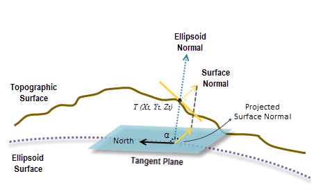
To calculate the aspect at each location, a quadratic or biquadratic surface is fitted to the neighborhood cells using the Least Squares Method (LSM). A surface normal is calculated at the cell location from that surface. At the same location, an ellipsoid normal perpendicular to the tangent plane of the ellipsoid surface is also calculated.

Since the tangent plane of the ellipsoid surface is considered the reference plane, the surface normal is projected onto the plane. Finally, the geodesic aspect is calculated by measuring the angle α in the clockwise direction between north and the projection of the surface normal (see the illustration above).

Slope

The Slope surface parameter is the steepness at each cell of a raster surface. The lower the slope value, the flatter the terrain; the higher the slope value, the steeper the terrain.

The output slope raster can be calculated in either of two units, degrees or percent (percent rise). The percent rise is better understood if you consider it as the rise divided by the run, multiplied by 100. Consider triangle B below. When the angle is 45 degrees, the rise is equal to the run, and the percent rise is 100 percent. As the slope angle approaches vertical (90 degrees), as in triangle C, the percent rise begins to approach infinity.

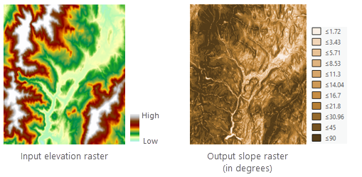
Slope is most frequently run on an elevation dataset as the following images show. Steeper slopes are shaded darker brown on the output slope raster.

The tool can also be used with other types of continuous data, such as population, to identify sharp changes in value.

Geodesic slope calculations

The geodesic slope is the angle formed between the topographic surface and the ellipsoid surface. Any surface parallel to the ellipsoid surface has a slope of 0. To calculate the slope at each location, a quadratic or biquadratic surface is fitted to the neighborhood cells using the Least Squares Method (LSM). A surface normal is calculated at the cell location from that surface. At the same location, an ellipsoid normal perpendicular to the tangent plane of the ellipsoid surface is also calculated. The slope, in degrees, is calculated from the angle between the ellipsoid normal and the topographic surface normal. This angle is the same as between the topographic surface and the ellipsoid surface.

Overview of surface curvature

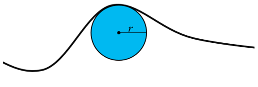
Curvature is a collection of surface parameter types used to describe the shape of a surface, typically along a line on the surface, created by the intersection of a plane through the surface. Conceptually, geometric curvature finds the best fitting circle (osculating circle) to approximate the shape of the curve at any point. The curvature is the reciprocal of the radius of that circle (1/r). A straighter line will be best fit with a larger circle resulting in a smaller curvature, and tighter curved line will be best fit with a smaller circle resulting in a larger curvature (Crane, 2018).

Profile (normal slope line) curvature

The Profile (normal slope line) curvature surface parameter measures the geometric normal curvature along the slope line. Sometimes referred to as profile curvature, it can be visualized as the shape of a vertical (profile) cross section through the surface. As illustrated below, the vertical plane cuts through the surface along the orange line, and if cut away, would appear as a cross-sectional profile of the surface.

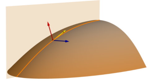
That plane is defined by two vectors, the yellow arrow showing gradient direction or slope line arrow, and the red arrow indicating the surface normal. It is the combination of these red and yellow vectors that define the orange plane and its orange line of intersection with the surface. The profile curvature is computed along the orange line (normal slope line) in the orange plane.

The normal slope line terminology of Minár et al (2020) is used here to minimize ambiguity and confusion with earlier terminology.

This curvature is typically applied to characterize the acceleration and deceleration of flow down the surface by force of gravity. At higher velocity, water can carry and move larger amounts of material; areas of acceleration become areas of erosion and areas of deceleration become areas of deposition.

In the image below, areas of high convex profile (normal slope line) curvature around the ridge of the cone are show in purple. Areas of high concave profile (normal slope line) curvature at the base of the cone are shown in orange. Areas with small curvature values are transparent.

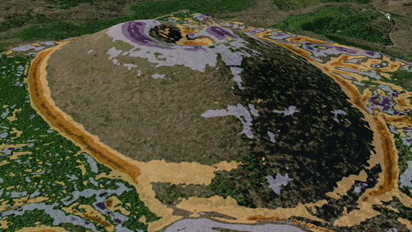
Results of this curvature are different from the Profile curvature output from the previous Curvature tool. An explanation of the differences between Profile curvature and Profile (slope line) curvature is provided later.

The formula for calculating profile (normal slope line) curvature is as follows:

• Where:

  K_P = Profile (normal slope line) curvature

  z = f(x,y)

Tangential (normal contour) curvature

The Tangential (normal contour) curvature surface parameter measures the geometric normal curvature perpendicular to the slope line, tangent to the contour line. It is referred to as the tangential curvature because it measures the curvature tangent to the contour line. It is described as normal contour (Minár et al., 2020) because the purple cutting plane that creates the purple line the curvature is computed along is defined by the blue contour vector and the red surface normal vector.

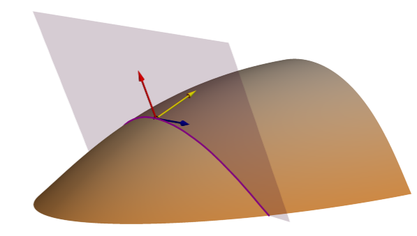
Tangential (normal contour) curvature is typically applied to characterize topographic convergence and divergence of flow across the surface.

In the image below, areas of high convex tangential (normal contour) curvature around the ridge of the cone, and ridge facing toward you, are show in blue. These are areas of diverging flow. Areas of high concave tangential (normal contour) curvature inside the cone show converging flow in red. Areas with small curvature values are transparent.

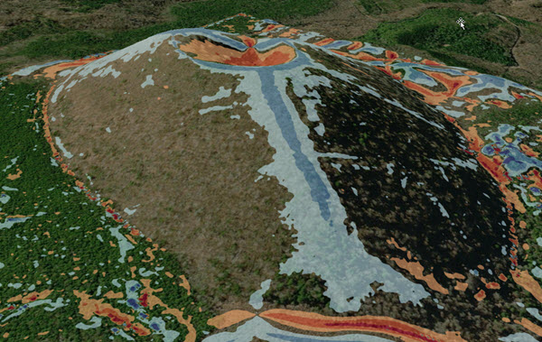
The formula for calculating tangential (normal contour) curvature is as follows:

• Where:

  K_T = Tangential (normal contour) curvature

  z = f(x,y)

Plan (projected contour) curvature

The Plan (projected contour) curvature surface parameter measures the curvature along contour lines. It is sometimes referred to as contour curvature and horizontal curvature. Projected contour curvature is measured along the contour line in blue, where the horizontal plane intersects the surface.

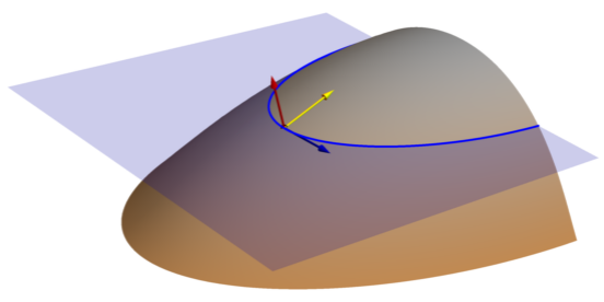
The formula for calculating Plan (projected contour) curvature is as follows:

• Where:

  K_PC = Plan (projected contour) curvature

  z = f(x,y)

The image below illustrates the difference between Tangential (normal contour) curvature, measured along the purple line, and Plan (projected contour) curvature, measured along the blue contour line.

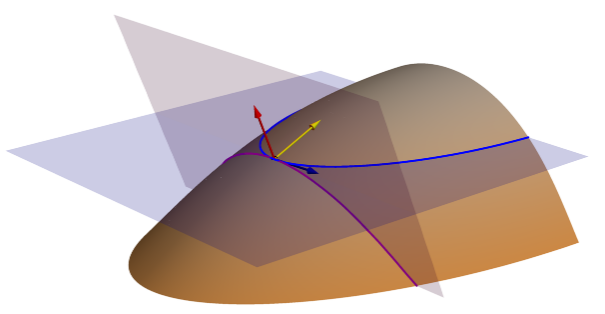
Contour geodesic torsion

The Contour geodesic torsion surface parameter measures the rate of change in slope angle along contour lines.

The formula for calculating Contour geodesic torsion is as follows:

• Where:

  τ = Contour geodesic torsion

  z = f(x,y)

Mean curvature

The Mean curvature surface parameter measures the overall curvature of the surface. It is computed as the average of the minimum and maximum curvature. It is also mathematically equivalent to the mean of the Profile (normal slope line) and Tangential (normal contour) curvatures. In the image below, the Profile (normal slope line) cutting plane (orange) and the Tangential (normal contour) cutting plane (purple) are shown.

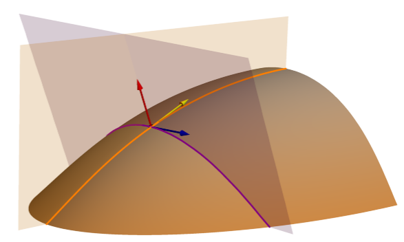
Profile (normal slope line) and Tangential (normal contour) curvature each measure convexity and concavity in a specific direction; whereas, Mean curvature describes the intrinsic convexity or concavity of the surface, independent of direction or gravity influence. Its sign (positive or negative) is not a definitive indicator of convexity or concavity except at extreme values, since a surface can be concave in one direction while also convex in another. High positive values indicate areas of maximum denudation, and high negative values indicate areas of maximum accumulation (Minár et al., 2020).

The formula for calculating Mean curvature is as follows:

• Where:

  K_M = Mean curvature

  z = f(x,y)

Gaussian curvature

The Gaussian curvature surface parameter measures general curvature of a surface. It is computed as the product of the minimum and maximum curvature and can take negative and positive values. Positive values indicate that the surface is convex at that cell, and negative values indicate that it is concave. A value of 0 indicates that the surface is flat.

The formula for calculating Gaussian curvature is as follows:

• Where:

  K_G = Gaussian curvature

  z = f(x,y)

Casorati curvature

The Casorati curvature surface parameter measures general curvature of the surface. It can be zero or any other positive number. High positive values indicate areas of sharp bending in multiple directions.

The formula for calculating Casorati curvature is as follows:

• Where:

  K_C = Casorati curvature

  z = f(x,y)

Basic and combinatorial curvature types

Tangential (normal contour) curvature, Profile (normal slope line) curvature, and Contour geodesic torsion are considered basic curvature types because other curvatures can be expressed as a combination of them. Adopting the terminology of Minár et al (2020), they are described as the Basic trio.

In addition to the expressions provided above for Mean curvature, Gaussian curvature, and Casorati curvature, these curvatures can also be computed as a combination of the Basic trio.

The formula for calculating Mean curvature is as follows:

• Where:

  K_M = Mean curvature

  K_T = Tangential (normal contour) curvature

  K_P = Profile (normal slope line) curvature

  z = f(x,y)

The formula for calculating Gaussian curvature is as follows:

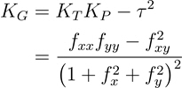
• Where:

  K_G = Gaussian curvature

  K_T = Tangential (normal contour) curvature

  K_P = Profile (normal slope line) curvature

  τ = Contour geodesic torsion

  z = f(x,y)

The formula for calculating Casorati curvature is as follows:

• Where:

  K_C = Casorati curvature

  K_M = Mean curvature

  K_G = Gaussian curvature

  z = f(x,y)

Comparison to legacy Curvature tool algorithms

The Surface Parameters tool uses different curvature algorithms than the Curvature tool, as well as geodesic math in its calculations; therefore, no direct comparison of outputs between these two tools should be made. The Surface Parameters curvature types, Profile (normal slope line) and Tangential (normal contour), are true geometric curvatures (Minár et al. 2020). The Surface Parameters tool's Mean curvature is the average of the minimum and maximum curvature at that point. The Profile and Planform types of the Curvature tool are directional derivatives, not actually measuring the geometric curvature of the surface at a location (Zevenbergen and Thorne 1987). The sign (positive or negative) for Profile (normal slope line) in the Surface Parameters tool is opposite of the Profile curvature of the Curvature tool. The Surface Parameters tool computes in geodesic space, and the Curvature tool uses planar coordinates and math. The Surface Parameters tool can fit either a quadratic or biquadratic surface, the Curvature tool only supports biquadratic.

Neighborhood distance

The Neighborhood distance value is the map distance from the center of the current processing cell to the center of an orthogonal neighbor. A smaller neighborhood distance captures more local variability in the landscape, which yields characteristics of smaller landscape features. With higher resolution elevation data, a larger neighborhood distance may be more appropriate due to fine scale error (noise) in the data that is not reflective of the landform processes of interest or because the landform of interest is more recognizable at larger distances.

The example below used a 5 meter resolution digital surface model (DSM) that has noticeable noise and striping artifacts showing in the profile (normal slope line) curvature result. The first image used the default 3 x 3 window or 5 meter neighborhood distance, the second image is a 9 x 9 cell window or 20 meter neighborhood distance, and the third image used a 15 x 15 cell window or 35 meter neighborhood distance. In this example, with increasing neighborhood distance, the most significant or primary features of the landscape become more clear, and the noise and striping artifacts are less visible. Although a larger neighborhood distance will always result in less noise, the most appropriate distance will depend on the cell size of the data and the size of landform features that are important for the application.

The smallest neighborhood distance is equal to the cell size of the input raster. The largest neighborhood distance is equal to seven times the cell size, resulting in a 15 x 15 cell window. Any specified distance that is larger than seven times the cell size will always result in using a 15 x 15 cell window.

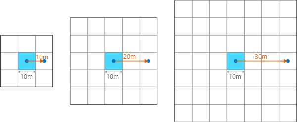
If a neighborhood distance is specified that does not result in an odd interval of the cell size, it will round up to the next interval of the cell size. For example, in the illustration above, if a neighborhood distance of 25 meters was specified, it will round up to the next interval of the cell size, 30 meters (three times the cell size), resulting in a 7 x 7 cell window.

If the elevation data is much finer spatial resolution than necessary for analyzing the landforms of interest, an alternative to the neighborhood window option is to resample or aggregate the data to a larger cell size that is more appropriate for the application.

Surface parameter calculations are sensitive to cell size and neighborhood distance. Wilson (2018) and Minár et al (2020) provide effective, up-to-date summaries of the numerous studies on this topic.

Adaptive neighborhood

When checked, the Use adaptive neighborhood parameter changes the neighborhood distance (window size or area) used for computing the surface parameter to better capture relevant variation in the landscape. The tool automatically determines the appropriate window size by computing the local deviation from mean elevation (DEV) (Wilson and Gallant, 2000) based on the values of all cells within the neighborhood. It attempts to use the largest window size possible while minimizing surface variability (James et al., 2014). The largest window size used is specified in the Neighborhood distance parameter.

When computing the surface parameter with a fixed neighborhood, all cell values within the neighborhood are used. When computing the surface parameter with an adaptive neighborhood, only nine cells (the outer orthogonal and diagonal cells and center processing cell) of the neighborhood are used.

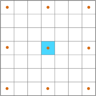
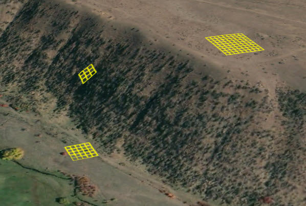
The adaptive neighborhood is particularly useful when analyzing a landscape with terrain features of widely varying size, such as large rolling hills with small gullies or stream channels, from a high resolution DEM. In such a situation, a small neighborhood distance such as 1 meter can be used for the creek gullies and larger neighborhood distance of 10 or 15 meters used for the hills.

In the illustration below, a smaller neighborhood is appropriate for the creek and edge of the cliff, a larger neighborhood for the transition from hill to plain, and an even larger neighborhood for the nearly flat homogeneous plateau.

Edge effect of neighborhood distance

Cells around the outer edge of the output will be assigned NoData when insufficient information is available for the calculation.

When using the adaptive neighborhood option, the extent of the output raster will shrink around its outer edge by one cell.

When using a fixed neighborhood distance larger than the input cell size, the output raster extent will be reduced according to the neighborhood distance used. The amount of reduction can be calculated as (window width in pixels - 1) / 2

For example, if the neighborhood distance results in using a window of 7 x 7 cells, the output raster will shrink around its outer edge by three cells.

Quadratic and biquadratic

There are two types of local surfaces that can be fit to the neighborhood window, quadratic and biquadratic. The default is quadratic and is recommended for most data and applications.

The quadratic surface is a least squares fit of the points and does not pass exactly through all points. By not passing exactly through all points, using the quadratic surface has the effect of minimizing the impact of noisy surface data such as a high resolution lidar surface. This creates a more representative result for all surface parameters and is especially important when computing curvature.

The quadratic surface should be used when specifying a neighborhood size that is larger than the cell size and when using the adaptive neighborhood option.

The biquadratic surface fits the data from the neighborhood cells exactly. This option is suitable for a highly accurate input surface free of random noise. If the neighborhood distance is larger than the input raster cell size, the accuracy advantages of the biquadratic surface type will be lost; therefore, neighborhood distance should be left as the default (equal to the cell size).

Geodesic coordinate transformation

The Surface Parameters tool performs its calculations in a geocentric 3D coordinate system—also called the Earth Centered, Earth Fixed (ECEF) coordinate system—by considering the shape of the earth as an ellipsoid. The computation result is not affected by how the dataset is projected. It will use the z-units of the input raster if they are defined in the spatial reference. If the spatial reference of the input does not define the z-units, you will need to do so with the z-unit parameter.

The ECEF coordinate system is a 3D right-handed Cartesian coordinate system with the center of the earth as the origin, where any location is represented by X, Y, and Z coordinates. See the following figure for an example of a target location T expressed with geocentric coordinates:

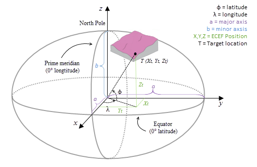
The surface raster is transformed from the input coordinate system into a 3D geocentric coordinate system.

The geodesic computation uses an X, Y, Z coordinate that is calculated based on its geodetic coordinates (latitude φ, longitude λ, height h). If the coordinate system of the input surface raster is a projected coordinate system (PCS), the raster is first reprojected to a geographical coordinate system (GCS) where each location has a geodetic coordinate. It is then transformed to the ECEF coordinate system. The height h (z-value) is the ellipsoid height referenced to the ellipsoid surface. See the illustration graphic below.

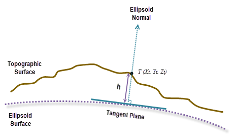
To transform to ECEF coordinates from a geodetic coordinate (latitude φ, longitude λ, height h), use the following formulas:

X = (N(φ) + h) * cos(φ) * cos(λ)

Y = (N(φ) + h) * cos(φ) * sin(λ)

Z = (b2 / a2 * N(φ) + h) * sin(φ)

• Where:

  N(φ) = a2 / √( a2 * cos(φ)2 + b2 * sin(φ)2)

  φ = latitude

  λ = longitude

  h = ellipsoid height

  a = major axis of the ellipsoid

  b = minor axis of the ellipsoid

The ellipsoid height h is in meters in the above formulas. If the input raster's z-unit is specified in any other unit, it will be internally transformed to meters.

Recommended reading

For a greater understanding of the surface analysis methods and their applications, see the references below. Additionally, Hengl and Reuter (2008), and Wilson (2018) both provide a comprehensive cataloging of these and many more terrain analysis techniques and their applications. Minár et al (2020) provides a comprehensive summary and comparison of prior work on land surface curvature, with clarity and definition of many types of curvature.

References

B. Hofmann-Wellenhof, H. Lichtenegger and J. Collins, 2001. GPS - theory and practice. Section 10.2.1. p. 282.

Burrough, P. A., and McDonell, R. A., 1998. Principles of Geographical Information Systems (Oxford University Press, New York), 190 pp.

Crane K., 2018. Discrete Differential Geometry: An Applied Introduction. Notices of the AMS, Communication. https://www.cs.cmu.edu/~kmcrane/Projects/DDG/paper.pdf

David Eberly 1999. Least Squares Fitting of Data (Geometric Tools, LLC), pp. 3.

E.J.Krakiwsky, and D.E.Wells, 1971. Coordinate Systems In Geodesy (GEODESY AND GEOMATICS ENGINEERING, UNB), LECTURE NOTES, No16, 1971, pp. 18-38

Hengl T. and Reuter H. 2008. Geomorphometry Concepts, Software, Applications. Elsevier.

James D.E., M.D. Tomer, S.A. Porter. 2014. Trans-scalar landform segmentation from high-resolution digital elevation models. Poster presented at: ESRI Annual Users Conference; July 2014; San Diego, CA.

Lancaster, P. and Šalkauskas, K. Curve and Surface Fitting: An Introduction. London: Academic Press, 1986.

Marcin Ligas, and Piotr Banasik, 2011. Conversion between Cartesian and geodetic coordinates on a rotational ellipsoid by solving a system of nonlinear equations (GEODESY AND CARTOGRAPHY), Vol. 60, No 2, 2011, pp. 145-159

Minár, J., Evans, I. S., & Jenčo, M. (2020). A comprehensive system of definitions of land surface (topographic) curvatures, with implications for their application in geoscience modelling and prediction. Earth-Science Reviews, 103414. https://doi.org/10.1016/j.earscirev.2020.103414

Wilson J.P and Gallant, J.C. (Eds.) 2000. Terrain Analysis: Principles and Applications. John Wiley & Sons, Inc.

Wilson J.P 2018. Environmental Application of Digital Terrain Modeling. John-Blackwell, Inc.

Zevenbergen, L. W., and C. R. Thorne. 1987. Quantitative Analysis of Land Surface Topography. Earth Surface Processes and Landforms 12: 47-56.