Composite indices are used across social and environmental domains to represent complex information from multiple indicators as a single metric that can measure progress toward a goal and facilitate decisions. The Calculate Composite Index tool supports the three main steps of the index creation process: standardize input variables to a common scale (preprocessing), combine variables to a single index variable (combination), and scale the resulting index to meaningful values (postprocessing).
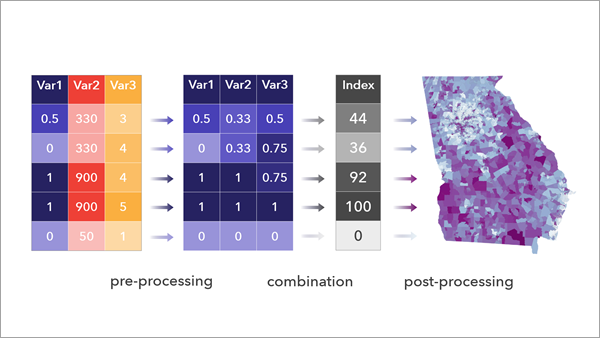
Design the index
Creating an appropriate index depends on careful consideration of the question the index is trying to answer, the variable choice, and the methods applied. Consulting with domain experts and end users is helpful.
Consider the following when designing the index:
- Whether to structure the variables into subindices. The concept that the index is measuring may be represented by multiple dimensions. For example, a vulnerability index might be composed of housing, transportation, and income domains, each comprising multiple variables. You can construct subindices to represent each dimension by running the tool multiple times. This can aid with interpretability, and depending on the methods used, it may also change the results of the index.
- How to select variables. A best practice is to reduce the number of input variables while keeping enough to capture the essential information needed for the index. A large number of input variables may result in difficulty when interpreting the index. Additionally, if multiple variables pertain to the same domain, for example, median income and poverty, the influence of this domain may be overrepresented in the index result. If this influence is unintended, this is known as unintentional weighting.
Learn more about best practices and important considerations in creating an appropriate index
Set variable weights
Variables are weighted to represent the relative importance of each factor as it contributes to the index. By default, all weights are set to 1, meaning that each variable is equally weighted. However, it may be important to denote differences in the relative contributions of a variable compared to the others. By changing one of the variables to a weight of 2 and keeping the others at 1, you denote that the variable should be considered twice as important as the others in its contribution to the final index.
You can also use weights that add up to 1. For example, if three variables are used and one should be considered twice as important as the other two, you can use weight values of 0.5, 0.25, and 0.25.
If variables are combined by mean, weights are applied by multiplying each variable by its respective weight. If weights are combined by geometric mean, weights are applied by raising each variable to the power of its respective weight.
Weights have a significant impact on the resulting index. Whether you keep equal weights or alter weights to favor variables, using weights adds subjectivity to the analysis. Additionally, you may unintentionally be weighting due to correlation and differences in variance between the variables.
Learn more about the impact of correlation and variance on the index
Preprocess variables
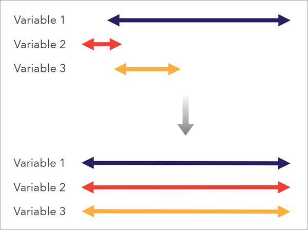
To create an appropriate index, variables must be in a compatible scale. To achieve this, preprocessing options are available in the tool that bring different input variables to a common measurement scale so they can be appropriately combined. You can also reverse variables so that the meaning of high values in each variable align with each other.
Preprocess variables to reverse direction
Consider the meaning of low and high values in each variable and ensure that they are consistent with each other. For example, in a social vulnerability index, locations with lower median incomes are more vulnerable, but locations with low percentages of people without insurance are less vulnerable; the direction of these variables are opposite in the context of the purpose of the index.
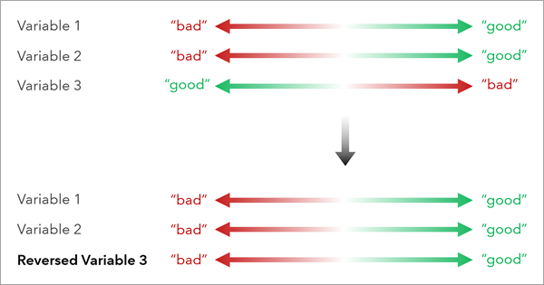
The reverse of the variable is calculated by multiplying each value by -1 and scaling the field between the original range of the variable.
Preprocess variables to use the same scale
The tool includes several options to scale the variables using the Method to scale and combine variables parameter. The Combine values (Mean of scaled values) and Compound differences (Geometric mean of scaled values) options scale using minimum-maximum values. The Combine ranks (Mean of percentiles) option scales using percentiles. The Highlight extremes (Count of values above 90th percentile) option scales using binary values. The selected option will be applied to all variables and the resulting scaled fields will be provided in the output. The following options are available:
Minimum-maximum—The variables are scaled between 0 and 1 using the minimum and maximum values of each variable. This method is the simplest, as it preserves the distribution of the input variables and scales to a 0 to 1 scale that is easy to interpret.
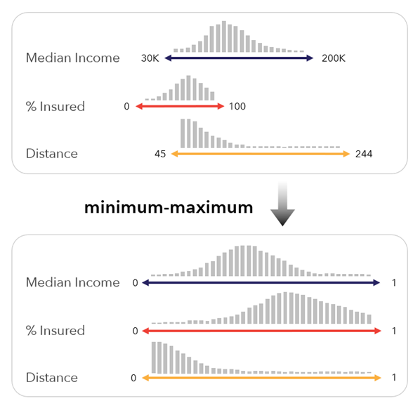
This method applies the following formula:

Since this method preserves the variable distribution, it can be affected by skewed distributions and outliers. For example, if there is a single outlier with a very high value, the outlier will receive a value of 1, but the rest of the values will be similar and closer to zero. Because of the reduced variation in the preprocessed variable, this variable may have less influence on the resulting index.
This method also depends on the minimum and maximum values in the input data, making it less appropriate for index comparisons across multiple time periods, when a variable's minimum and maximum values may change with each time step.
Percentile—The variables are converted to percentiles between 0 and 1. This method can be useful when the ranks of each variable are more important than their actual values. It is also robust to outliers and skewed distributions, as the variables are transformed to a uniform distribution.
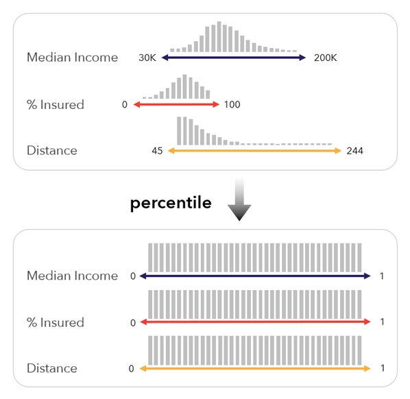
There are various definitions for percentiles. This method uses the following formula:
 ,
,where R is the ordinal rank (using the minimum rank value in the case of ties), N is the number of values, and P is the resulting percentile.
Percentiles denote the position of a value relative to the other values within the variable. For example, while the difference in income between $50,000 and $60,000 may not be substantial, the percentile difference may be large if there are many features with values in between.
Flag by threshold (binary)—The variable is converted to binary values (0, 1), which indicate whether the value is above or below a specified threshold. This method is useful when it is important to highlight certain values and the variation of the values does not matter.
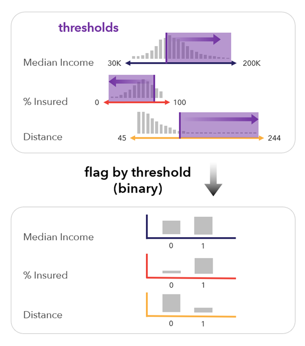
This method is not affected by outliers in the input variables, but the interval level information in each input variable is lost, as each variable is converted to a binary (0, 1) form.
- Raw—The original values of the variables are used. This method should only be used if all variables are on a comparable scale. For example, use this method when all variables are a standard unit such as percentages or parts per million. This method can also be useful when variable standardization or transformation has already occurred.
Combine variables
Once variables are preprocessed to a common scale, the variables are aggregated to create a single value. The Combine scaled values (Mean of scaled values) option of the Method to scale and combine variables parameter aggregates by mean. The Compound scaled values (Geometric mean of scaled values) method aggregates by geometric mean. The Highlight extremes (Count of values above 90th percentile) aggregates by sum.
Sum and Mean are additive methods. Geometric mean is a multiplicative method.
Additive methods
The Sum and Mean combination methods are relatively simple to interpret and are commonly used by a variety of indices. The methods are almost identical; they result in distributions with the same shape that only differ in scale, and the resulting index map will look the same. Only the values differ.
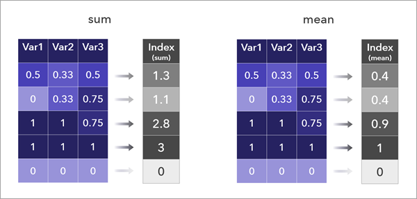
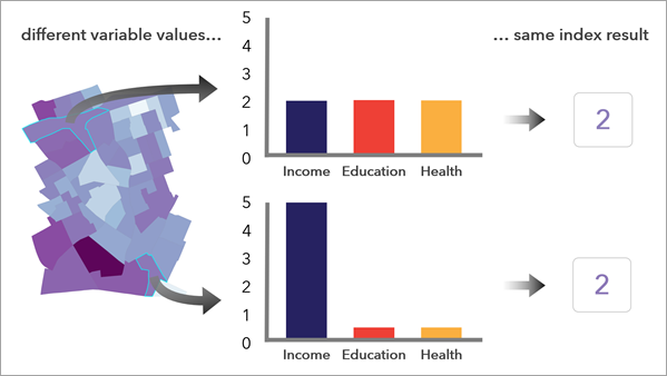
These methods allow high values in one variable to compensate for low values in another variable.
Multiplicative methods
Multiplicative methods have the advantage that they do not allow high values in one variable to compensate for low values in another variable; for an index value to be high, multiple variables must have high values.
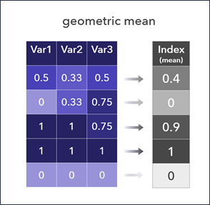
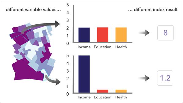
Geometric mean is similar to multiplication. An index using geometric mean will result in the same map as an index using multiplication to combine variables, as the distribution is the same shape, only the values differ.
Postprocess the index
Once variables are preprocessed and combined into the raw index, postprocessing may help make the index more understandable.
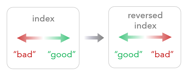
Reverse the index
Consider the purpose of the index, and evaluate whether high index values are as intended. Reversing the index will make high values in the raw index become low values in the final index and vice versa.
Scale the index using minimum and maximum values
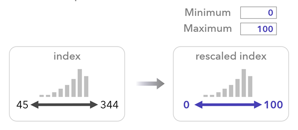
Using minimum and maximum values to scale the index changes the range of the output index. This option may be easier to interpret, regardless of the preprocessing and combination methods used. For example, specify a Minimum value of 0 and a Maximum value of 100 to scale the raw index to this range. This option uses the following formula:

where x is the original value, min(x) is the minimum value found in the index, max(x) is the maximum value found in the index, a is the specified minimum value, b is the specified maximum value, and x' is the scaled value.
Interpret results
The index layer displays the distribution of index values after any optional scaling or reversing. The layer provides a continuous choropleth map that can be used to evaluate the index results. You can use the map to evaluate high and low index values, preserving the index distribution and any outliers.
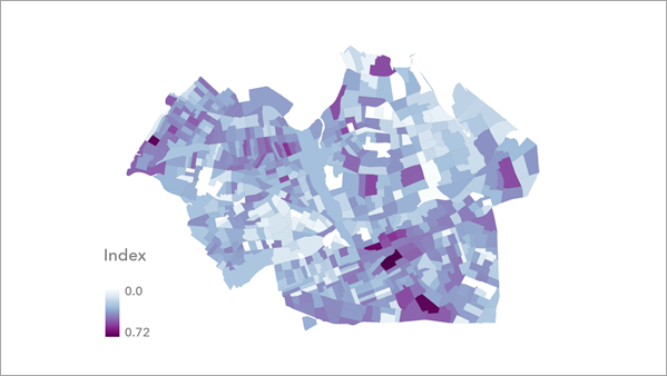
The layer also includes the following fields which can be used to explore the results:
- A percentile field which indicates the relative positions (ranks) between index values. Use this field to explore how locations relate to each other based on their rank instead of their actual index differences.
- A field with the index classified into five equal interval classes.
- A field with the index classified into five quantile classes.
- A field with the index classified into six standard deviation classes. Use this field to explore how the index value at each location relates to the mean index value and to identify locations with extremely high and low index values.
Additional resources
See the Organisation for Economic Co-operation and Development Handbook on Constructing Composite Indicators: Methodology and User Guide for additional information.