Available with Image Server
Once the adjusted straight-line distance is calculated, you can use the horizontal factor to control the rate at which the distance is encountered. You can use the cost surface, characteristics of the mover, and the vertical factor to control the rate as well.
The horizontal factor is the effort necessary to overcome, or the assistance gained by, an influence when moving through a landscape. Examples of a horizontal influence include wind if moving across land, and currents if the travel is across a body of water. The horizontal factor can affect how the distance is encountered. A cyclist pedaling into a head wind will exert more effort to overcome it or will cover distances at a slower rate. Pedaling with the wind requires less effort, and a cross wind is somewhere in between. Modifying the distance for this influence helps capture the rate at which the distance is encountered by the traveler.

If the wind is blowing behind the cyclist at a 45-degree angle offset, the wind will be of some advantage to the cyclist but not as much as if blowing directly behind (a 0-degree offset).

The horizontal factor (HF) is a multiplier modifier to the distance calculations.
The direction of the horizontal influence for each cell is identified in the horizontal raster. The horizontal factor will vary based on the direction the traveler is moving. Using the Travel direction source characteristic parameter, you can define whether the traveler is moving toward or away from a source. Moving toward or away from a source would change the direction the traveler enters a cell. The traveler then will encounter the horizontal influence at a different angle, resulting in a change in the horizontal factor multiplier. For more information regarding how the travel direction and horizontal factor interact to affect the cost distance, Incorporate wind into the analysis in the source characteristics topic.
Horizontal factor use examples
The horizontal factor can be used in various scenarios, such as the following:
- Identify the route a ship should take by accounting for the influence of ocean currents that may alter the path to take, assuming a constant current speed in the study area.
- Determine the difference in flight time of an airplane traveling from New York City to Los Angeles and from Los Angeles to New York City. Flying east to west will take longer since the airplane will be flying into headwinds as opposed to flying west to east, assuming a constant wind speed.
- Propose a hiking trail following contour lines as much as possible. Areas of steep slope will be either treated as barriers or used as an input to the cost friction raster to increase construction cost where the trail will run along a contour line but encounters a dangerously steep slope.
- Build a gravity-driven wastewater pipe in an area where the pipe will follow the steepest downslope direction
Incorporate a horizontal factor
Distance analysis can be divided conceptually into the following related functional areas:
- Calculate straight-line distance and optionally adjust the calculations with a barrier or surface raster.
- Once the straight-line distance is calculated, optionally determine the rate the distance will be encountered through a cost surface, source characteristics, a vertical factor, and a horizontal factor. Create the accumulative distance raster.
- Connect regions over the resulting accumulative distance surface using an optimal network, specific paths, or a corridor.
From the second functional area, determine the rate at which the distance will be encountered through a horizontal factor as illustrated below.
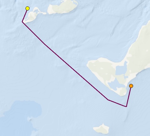
A boat is starting at a marina (the yellow point) and will travel to a second marina (the orange point). The purple line shows the shortest straight-line route to travel between the two marinas while traveling around the islands.
However, a current is moving from the northwest to the southeast (the grey polygon). Using the current, the magenta line is the fastest route to get from the first marina (the yellow point) to the second marina (the orange point).
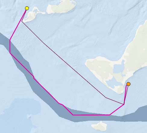
When a horizontal raster is incorporated, the direction of travel matters. In this example, the cost and route for moving from the first marina to the second marina is different than traveling from the second marina back to the first.
Create a distance map using a horizontal factor
To create a distance map that incorporates a horizontal factor, complete the following steps:
- Open the Distance Accumulation tool.
- Provide a source for the Input raster or feature source data parameter.
- Name the output distance raster.
- Expand the Costs relative to horizontal movement category.
- Provide a horizontal factor raster for the Input horizontal raster parameter.
This raster identifies the direction of the horizontal influence for each cell.
- Specify the Horizontal factor value.
This parameter identifies the multiplier to be applied to capture how the horizontal factor influences how the distance is encountered.
- Click Run.
Horizontal factor affects the rate distance is encountered
In order to modify the rate distance is encountered and account for the influence of the horizontal factor, internally the tool performs two actions:
- From the horizontal factor raster, calculate how the horizontal factor will be encountered when moving from one cell to the next. This is referred to as the horizontal relative moving angle (HRMA).
- Identify how the HRMA will modify the rate the distance is encountered
Calculate the HRMA
To calculate the total HF for traveling between cells, the HF from the processing cell (the From cell) to the edge of the cell you are calculating the distance for (the To cell) must be determined as well as the HF from the edge of the To cell to its center.
First, the horizontal direction must be established. Horizontal direction is measured in degrees from 0 to 360. The starting point is to the north of the processing cell, increasing in a clockwise direction.
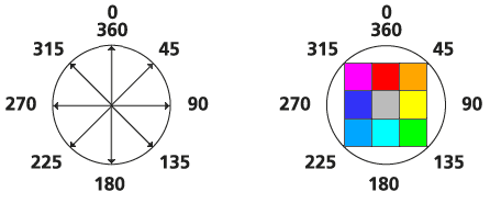
The horizontal direction is defined by the value assigned to each cell location on the input horizontal factor raster. It typically identifies the direction with the lowest horizontal cost of movement with respect to the processing cell.
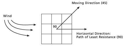
Once the horizontal direction has been defined, the position of the cell that is being moved into (the To cell) relative to the horizontal direction must be determined. The direction of the To cell relative to the prevailing horizontal direction at the processing cell is the horizontal moving direction. The angle of the To cell from the horizontal direction as defined by the horizontal factor raster is the HRMA.

The number of degrees from the established horizontal direction is what is relevant, not the side of the established direction.

Identify the HF multiplier
Once the HRMA has been determined, a graph is used to identify the horizontal factor multiplier. The HF is on the y-axis, and the HRMA is on the x-axis.
In the example above, the cell whose horizontal factor you are calculating has an HRMA of 90 degrees from the horizontal direction as defined by the processing cell on the input horizontal factor raster. If the Linear horizontal factor graph is used, the horizontal factor cost will be 1.61. In the graph below, at 90 on the x-axis, go up to the green function line, and follow the function line to the horizontal factor multiplier on the y-axis.
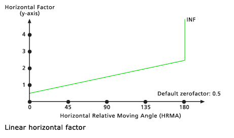
The HRMA values can range from -180 to 180 degrees. However, on the horizontal factor graph, only values from 0 to 180 are presented on the x-axis because the graph is assumed to be symmetrical (mirrored) around the horizontal factor axis. That is, an HRMA of 90 has the same horizontal factor as an HRMA of -90. INF means the line goes to infinity.
This same process is performed for the segment starting at the edge of the To cell and ending at its center. The moving direction remains the same, but the horizontal direction that will be used for the calculations is the prevailing horizontal direction at the To cell. Dividing the travel link between two cells into two segments (half the segment being in the processing cell and the other half in the To cell) provides a more accurate horizontal factor. When leaving the processing cell, the traveler encounters the horizontal factor associated with the processing cell. When the traveler moves into the To cell, they encounter the horizontal factor associated with the To cell. In the distance formula, each segment's horizontal factor is multiplied by its respective cost, which is determined from the cost raster if one has been entered.
The horizontal factor functions that allow you to capture the interaction of the traveler to the horizontal factor influences they are encountering are Binary, Forward, Linear, Inverse linear, and Table.
Note:
The horizontal factor is a multiplier. Take care when specifying the units when combining the horizontal factor with a cost surface, source characteristics, or a vertical factor. Generally, when a cost surface is entered, the horizontal factor should be a multiplier adjustment of the rate of cost surface units. If time is the unit for the rate of the cost surface, the horizontal factor should be a modifier of time. Only one of these factors can define the units for the rate. The other factors are unitless, and their values are multiplier modifiers of the specified units.
Sample application that uses a horizontal factor
A sample application that uses a horizontal factor is described below.
Use a horizontal factor for trail construction
You want to construct a trail extension between two existing trailheads. You want the trail to follow contour lines as closely as possible, so that trail users don’t have to travel uphill or downhill more than necessary. In the image below, the first attempt at this is shown by the red route. That route has some shortcomings. It traverses exposed rock faces, which will be expensive to construct and maintain. The trail may then be highly visible, and construction will have a high environmental impact. The second attempt, shown by the yellow route, is more reasonable. A cost surface was used as input to the analysis, which increases the cost of trail construction in high-slope areas.
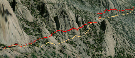
The horizontal factor raster for both routes is created from a 1-meter resolution elevation surface using the Surface Parameters tool. A temporary aspect raster was created that shows the direction of maximum human scale slope (roughly 5 meters). Then map algebra was applied to rotate the aspect azimuths 90 degrees. The result is a horizontal factor raster that identifies the direction of the contour lines at each cell. Finally, a symmetric horizontal factor function was used to restrict motion that is not in the direction of the contour lines.
For the yellow route, a cost surface was input that hinders trail construction in high slope areas.
Additional information
The following sections provide additional information regarding horizontal factors.
Horizontal factors
To define the horizontal factor function that will be used to determine the horizontal factor multiplier, you can choose an existing function from the graphs provided with the software or you can create a custom function using an ASCII file. The following horizontal factor functions, are available in the Distance Accumulation and Distance Allocation tools:
Horizontal factor options, modifiers, and default values
| Function | Zero factor | Cut angle | Slope | Side value |
|---|---|---|---|---|
Binary | 1 | 45 | N/A | N/A |
Forward | 0.5 |
N/A | N/A | 1 |
Linear | 0.5 | 181 | 1.111E-02 | N/A |
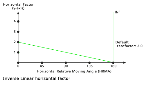
Inverse linear | 2 | 180 | -1.111E-02 | N/A |
The following is a description of each horizontal factor function. Each function can be further refined through a series of modifiers. The modifiers are described in the following section.
Binary
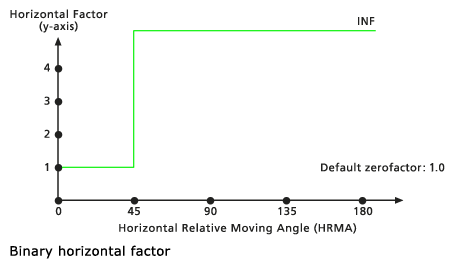
When the HRMA is less than the cutting angle, the HF for moving through the section of the cell is set to the value of Zero factor. If the HRMA is greater than the cutting angle, the HF for the section is set to infinity. The default cutting angle is 45 degrees. The default zero factor is 1.0.
Forward
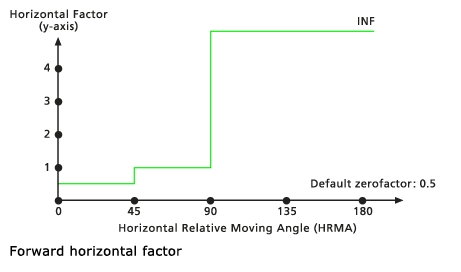
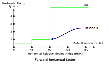
If an HRMA is less than 45 degrees for a section of travel, the HF is set to the value of Zero factor. When the HRMA is larger than or equal to 45 degrees and less than 90 degrees, the HF is set to the value of Side value. If no side value is specified, the default side value is 1. If the HRMA is equal to or greater than 90 degrees, the HF is set to infinity. The default zero factor is 0.5.
Linear
The HFs are determined by a straight line in the HRMA-HF coordinate system. The line intercepts the y-axis, equitable to the HF factor, at the Zero factor value. The slope of the line can be specified using the Slope modifier. If no slope is identified, the default is 0.5/45 or 1/90 (specified as 0.01111). The default cutting angle is 181 degrees, which equates to no cutting. The default zero factor is 0.5.

Inverse linear
The HFs are determined by the inverse values from a straight line in the HRMA-HF coordinate system. The line intercepts the y-axis, equitable to the HF factor, at the Zero factor value. The slope of the line can be specified with the Slope modifier. If no slope is identified, the default is -2/180 or -1/90 (specified as 0.01111). The default cutting angle is 181 degrees, which equates to no cutting. The default zero factor is 2.0.
Table
A graph can be defined with an ASCII file created in any text editor. The file consists of two columns of values on each line. The first value identifies the HRMA, which is expressed in degrees, and the second column identifies the HF. Each line specifies a point on the graph. Two consecutive points define a line segment in the HRMA-HF coordinate system. The HRMA angles must be entered in ascending order. The HF factor for any HRMA angle less than the first (lowest) input value or larger than the last (largest) input value will be set to infinity. An infinite HF is represented by -1 in the ASCII file.
The following is a sample horizontal factor ASCII table:
    0    1.40
    10   2.43
    20   2.30
    30   3.44
    40   1.25
    50   1.02
    60   0.90
    70   0.86
    80   0.25
    90   0.78
    100  1.49
    110  2.35
    120  3.32
    130  2.39
    140  3.18
    150  2.13
    160  1.89
    170  1.20
    180  2.034
Horizontal factor modifiers
Several of the HRMA keyword parameters have modifiers that can be specified to achieve various results. The slope of the line in the Linear and Inverse linear functions, the side values for the Forward function, and the zero factor can alter the y-axis intercept for the input functions, and the cut angle for any of the HRMA functions can be controlled.
Zero factor
This modifier positions the y-intercept of the specified function. It can be used in conjunction with all horizontal factor functions.
Cut angle
This modifier establishes the HRMA degree threshold beyond which the HFs are set to infinity. Cut angle can be used on any of the specified horizontal factor keywords except Forward. That function, by definition, establishes its own cut angles.
Slope
This modifier identifies the slope of the straight lines in the HRMA–HF coordinate system for the Linear and Inverse linear keywords. Slope is specified as the rise over the run (for example, a 30-degree slope is 1/30, specified as 0.03333). See the Linear HRMA diagram for an example of a line with a slope of 1/90.
Side value
This modifier identifies the HF value that will be assigned for HRMAs that are equal to or less than 45 degrees and less than 90 degrees when the Forward horizontal factor keyword is used. Review the Forward HRMA diagram, which has a side value of 1.
Table name
This modifier identifies the name of the ASCII file that will be used for the Table option.